SVM

What is SVM

The objective of the support vector machine algorithm is to find a hyperplane in an N-dimensional space(N — the number of features) that distinctly classifies the data points. To separate the two classes of data points, there are many possible hyperplanes that could be chosen. The objective is to find a plane that has the maximum margin, i.e the maximum distance between data points of both classes. Maximizing the margin distance provides some reinforcement so that future data points can be classified with more confidence.Support vectors are data points that are closer to the hyperplane and influence the position and orientation of the hyperplane. Using these support vectors, the margin of the classifier is maximized.

SVM in R

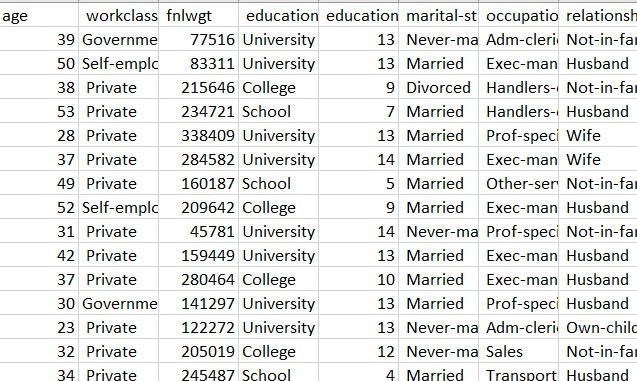
The SVM is created using record dataset in R. It is the same record dataset used for naive bayes. The dataset has been downloaded from UCI Machine learning repository. The link for the source can be found here This dataset consists of various features like age, workclass, education, marital status, relationship, race, sex, hours per week. The label column contains the data of whether the person is rich (salary greater than or equal to 50k) or poor(salary less than $50k).

Cleaning and formatting the dataset to the required format

The code to create clean and format the datasets can be found here

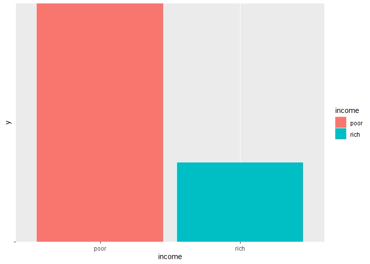
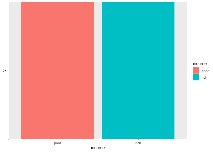
There are a lot of unwated columns in the dataframe. These columns are dropped from the dataframe, retaining only the necessary columns. The dataset is checked for NA values, and all the NA values are removed. Checking the balance of the dataset and label is very important before performing decision trees, as unbalanced dataset may lead to over or underfitting.

Model Building

The code to build the model can be found here

Before building the model, the dataset is split into training and testing sets. The split ratio is 0.75 of the total data in the training set and 0.25 data in the testing set. The SVM model is trained using the training dataset and then the model is tested using labels from the testing dataset. Three SVM models are created. The SVM models differ due to hypertuning of different parameters. Mainly the cost and kernel. The three types of kernel are polynomial, linear and radial. The cost is selected by tuning it for every kernel and selecting the best cost for each model.

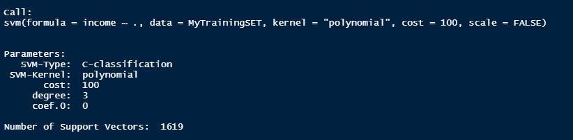
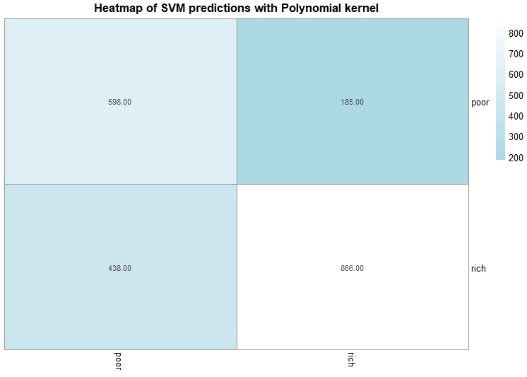
SVM Model 1

This is the first SVM Model. In this model, the kernel is polynomial and the best cost after tuning is 100. The accuracy of this model is 70%.

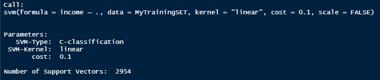
SVM Model 2

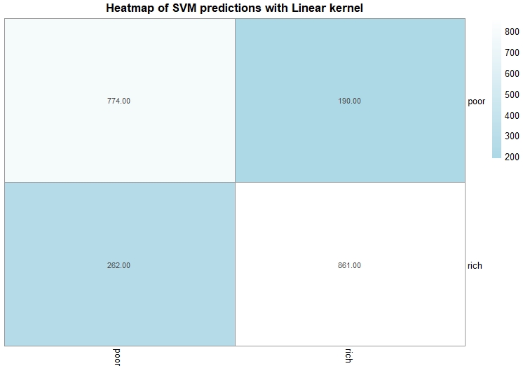
This is the second SVM Model. In this model, the kernel is linear and the best cost after tuning is 0.1. The accuracy of this model is 78%.

SVM Model 3

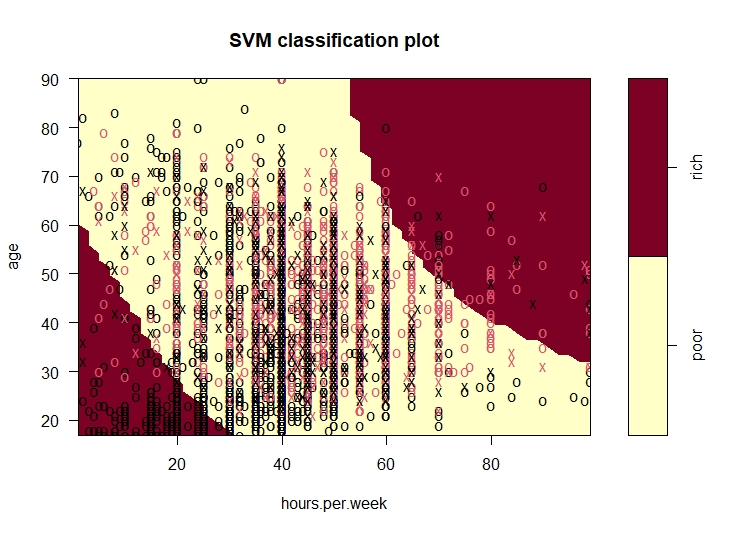
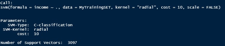
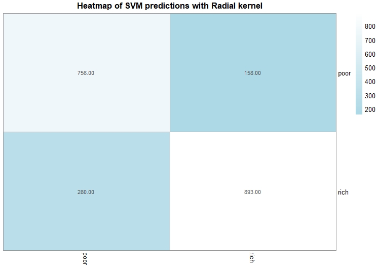
This is the third SVM Model. In this model, the kernel is radial and the best cost after tuning is 10. The accuracy of this model is 79%.

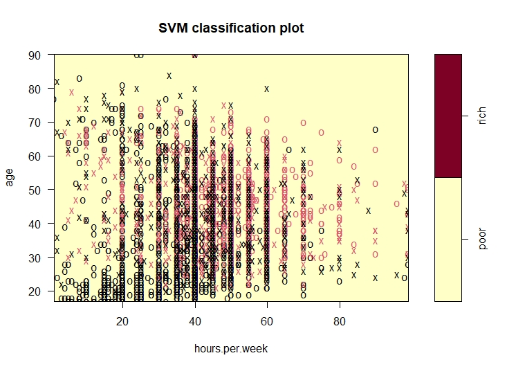
Conclusion

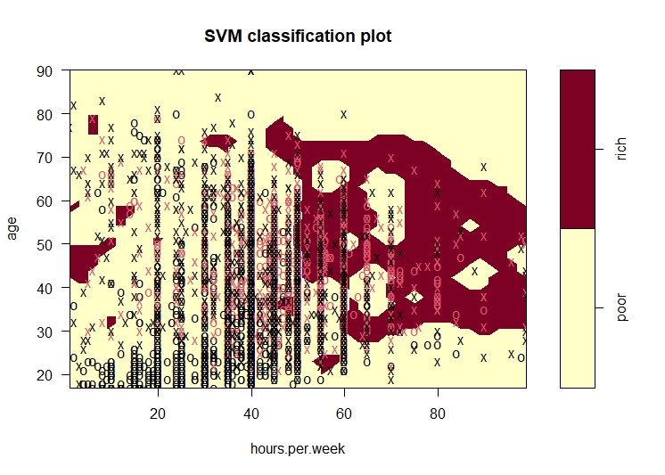
The intention was to perform svm to help predict the income class of a person given the different features. The accuracy of the models are in the range of 70-79% which is pretty decent in predicting the income group. The last model,i.e, the radial model is the best model for this data as it has the highest accuracy (79%). One of the plot for each model is created using the age and hours worked per week variable.